Till now, We have read about Gradient Descent,Min-Batch Gradient Descent,Stochastic Gradient Descent and other type of Gradient Descents and Polynomial Regression. In this post we will learn about Learning Curves in Machine Learning .
Introduction
Learning curves are graphical representations of how a model’s performance changes over time as it learns from training data. These curves are valuable tools for understanding the behavior of machine learning models, identifying issues such as overfitting or underfitting, and making informed decisions about model improvement.
If you perform high-degree Polynomial Regression, you will likely fit the training data much better than with plain Linear Regression. For example, Figure below applies a 300-degree polynomial model to the preceding training data, and compares the result with a pure linear model and a quadratic model (2nd-degree polynomial).
Notice how the 300-degree polynomial model wiggles around to get as close as possible to the training instances.

Of course, this high-degree Polynomial Regression model is severely overfitting the training data, while the linear model is underfitting it. The model that will generalize best in this case is the quadratic model. It makes sense since the data was generated using a quadratic model, but in general you won’t know what function generated the data, so how can you decide how complex your model should be? How can you tell that your model is overfitting or underfitting the data
We use cross-validation to get an estimate of a model’s generalization performance. If a model performs well on the training data but generalizes poorly according to the cross-validation metrics, then your model is overfitting. If it performs poorly on both, then it is underfitting. This is one way to tell when a model is too simple or too complex.
Another way is to look at the learning curves: these are plots of the model’s performance on the training set and the validation set as a function of the training set size (or the training iteration). To generate the plots, simply train the model several times on different sized subsets of the training set. The following code defines a function that plots the learning curves of a model given some training data:
Implementation
from sklearn.metrics import mean_squared_error
from sklearn.model_selection import train_test_split
def plot_learning_curves(model, X, y):
 X_train, X_val, y_train, y_val = train_test_split(X, y, test_size=0.2)
 train_errors, val_errors = [], []
 for m in range(1, len(X_train)):
 model.fit(X_train[:m], y_train[:m])
 y_train_predict = model.predict(X_train[:m])
 y_val_predict = model.predict(X_val)
 train_errors.append(mean_squared_error(y_train[:m], y_train_predict))
 val_errors.append(mean_squared_error(y_val, y_val_predict))
plt.plot(np.sqrt(train_errors), "r-+", linewidth=2, label="train")
plt.plot(np.sqrt(val_errors), "b-", linewidth=3, label="val")
Let’s look at the learning curves of the plain Linear Regression model (a straight line)
lin_reg = LinearRegression()
plot_learning_curves(lin_reg, X, y)

This deserves a bit of explanation. First, let’s look at the performance on the training data: when there are just one or two instances in the training set, the model can fit them perfectly, which is why the curve starts at zero. But as new instances are added to the training set, it becomes impossible for the model to fit the training data perfectly, both because the data is noisy and because it is not linear at all. So the error on the training data goes up until it reaches a plateau, at which point adding new instances to the training set doesn’t make the average error much better or worse. Now let’s look at the performance of the model on the validation data. When the model is trained on very few training instances, it is incapable of generalizing properly, which is why the validation error is initially quite big. Then as the model is shown more training examples, it learns and thus the validation error slowly goes down. However, once again a straight line cannot do a good job modeling the data, so the error ends up at a plateau, very close to the other curve.
These learning curves are typical of an underfitting model. Both curves have reached a plateau; they are close and fairly high.
If your model is underfitting the training data, adding more train‐
ing examples will not help. You need to use a more complex model
or come up with better features
Now let’s look at the learning curves of a 10th-degree polynomial model on the same data
from sklearn.pipeline import Pipeline
polynomial_regression = Pipeline([
 ("poly_features", PolynomialFeatures(degree=10, include_bias=False)),
 ("lin_reg", LinearRegression()),
 ])
plot_learning_curves(polynomial_regression, X, y)
These learning curves look a bit like the previous ones, but there are two very important differences:
- The error on the training data is much lower than with the Linear Regression model.
- There is a gap between the curves. This means that the model performs significantly better on the training data than on the validation data, which is the hall‐mark of an overfitting model. However, if you used a much larger training set, the two curves would continue to get closer.

One way to improve an overfitting model is to feed it more training
data until the validation error reaches the training error
The Bias/Variance Tradeoff
An important theoretical result of statistics and Machine Learning is the fact that a model’s generalization error can be expressed as the sum of three very different errors:
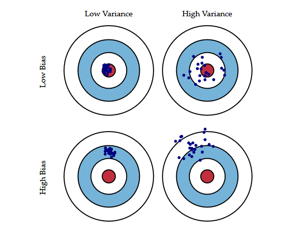
Bias
This part of the generalization error is due to wrong assumptions, such as assuming that the data is linear when it is actually quadratic. A high-bias model is most likely to underfit the training data.
Variance
This part is due to the model’s excessive sensitivity to small variations in the training data. A model with many degrees of freedom (such as a high-degree polynomial model) is likely to have high variance, and thus to overfit the training data.
Irreducible error
This part is due to the noisiness of the data itself. The only way to reduce this part of the error is to clean up the data (e.g., fix the data sources, such as brokensensors, or detect and remove outliers). Increasing a model’s complexity will typically increase its variance and reduce its bias. Conversely, reducing a model’s complexity increases its bias and reduces its variance. This is why it is called a tradeoff.
Important Notice for college students
If you’re a college student and have skills in programming languages, Want to earn through blogging? Mail us at geekycomail@gmail.com
For more Programming related blogs Visit Us Geekycodes . Follow us on Instagram.