Kernel PCA in Machine Learning

A mathematical technique that implicitly maps instances into a very high-dimensional space (called the feature space), enabling nonlinear classification and regression with Support Vector Machines. Recall that a linear decision boundary in the high-dimensional feature space corresponds to a complex nonlinear decision boundary in the original space. It turns out that the same trick can be applied to PCA, making it possible to perform complex nonlinear projections for dimensionality reduction. This is called Kernel PCA (kPCA).It is often good at preserving clusters of instances after projection, or sometimes even unrolling datasets that lie close to a twisted manifold. For example, the following code uses Scikit-Learn’s KernelPCA class to perform kPCA with an RBF kernel (see Chapter 5 for more details about the RBF kernel and the other kernels):

from sklearn.decomposition import KernelPCA
rbf_pca = KernelPCA(n_components = 2, kernel="rbf", gamma=0.04)
X_reduced = rbf_pca.fit_transform(X)

Figure below shows the Swiss roll, reduced to two dimensions using a linear kernel (equivalent to simply using the PCA class), an RBF kernel, and a sigmoid kernel (Logistic).

Selecting a Kernel and Tuning Hyperparameters

As kPCA is an unsupervised learning algorithm, there is no obvious performance measure to help you select the best kernel and hyperparameter values. However, dimensionality reduction is often a preparation step for a supervised learning task (e.g., classification), so you can simply use grid search to select the kernel and hyperparameters that lead to the best performance on that task. For example, the following code creates a two-step pipeline, first reducing dimensionality to two dimensions using kPCA, then applying Logistic Regression for classification. Then it uses Grid SearchCV to find the best kernel and gamma value for kPCA in order to get the best classification accuracy at the end of the pipeline:

from sklearn.model_selection import GridSearchCV
from sklearn.linear_model import LogisticRegression
from sklearn.pipeline import Pipeline
clf = Pipeline([
 ("kpca", KernelPCA(n_components=2)),
 ("log_reg", LogisticRegression())
 ])
param_grid = [{
 "kpca__gamma": np.linspace(0.03, 0.05, 10),
 "kpca__kernel": ["rbf", "sigmoid"]
 }]
grid_search = GridSearchCV(clf, param_grid, cv=3)
grid_search.fit(X, y)

The best kernel and hyperparameters are then available through the best_params_ variable:

print(grid_search.best_params_)
{'kpca__gamma': 0.043333333333333335, 'kpca__kernel': 'rbf'}

Another approach, this time entirely unsupervised, is to select the kernel and hyperparameters that yield the lowest reconstruction error. However, reconstruction is not as easy as with linear PCA. Here’s why. Figure 8-11 shows the original Swiss roll 3D dataset (top left), and the resulting 2D dataset after kPCA is applied using an RBF kernel (top right). Thanks to the kernel trick, this is mathematically equivalent to mapping the training set to an infinite-dimensional feature space (bottom right) using the feature map φ, then projecting the transformed training set down to 2D using linear PCA. Notice that if we could invert the linear PCA step for a given instance in the reduced space, the reconstructed point would lie in feature space, not in the original space (e.g., like the one represented by an x in the diagram). Since the feature space is infinite-dimensional, we cannot compute the reconstructed point, and therefore we cannot compute the true reconstruction error. Fortunately, it is possible to find a point in the original space that would map close to the reconstructed point. This is called the reconstruction pre-image. Once you have this pre-image, you can measure its squared distance to the original instance. You can then select the kernel and hyperparameters that minimize this reconstruction pre-image error.

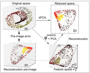
You may be wondering how to perform this reconstruction. One solution is to train a supervised regression model, with the projected instances as the training set and the original instances as the targets. Scikit-Learn will do this automatically if you set fit_inverse_transform=True, as shown in the following code:

rbf_pca = KernelPCA(n_components = 2, kernel="rbf", gamma=0.0433,
 fit_inverse_transform=True)
X_reduced = rbf_pca.fit_transform(X)
X_preimage = rbf_pca.inverse_transform(X_reduced)

By default, fit_inverse_transform=False and KernelPCA has no inverse_transform() method. This method only gets created when you set fit_inverse_transform=True.

You can then compute the reconstruction pre-image error:

from sklearn.metrics import mean_squared_error
mean_squared_error(X, X_preimage)
32.786308795766132

Conclusion

Now you can use grid search with cross-validation to find the kernel and hyperparameters that minimize this pre-image reconstruction error.