Using Clustering for Semi-Supervised Learning

Another use case for clustering is in semi-supervised learning, when we have plenty of unlabeled instances and very few labeled instances. Let’s train a logistic regression model on a sample of 50 labeled instances from the digits dataset:

n_labeled = 50
log_reg = LogisticRegression()
log_reg.fit(X_train[:n_labeled], y_train[:n_labeled])

What is the performance of this model on the test set?

log_reg.score(X_test, y_test)
0.8266666666666667

The accuracy is just 82.7%: it should come as no surprise that this is much lower than
earlier, when we trained the model on the full training set. Let’s see how we can do
better. First, let’s cluster the training set into 50 clusters, then for each cluster let’s find
the image closest to the centroid. We will call these images the representative images:

k = 50
kmeans = KMeans(n_clusters=k)
X_digits_dist = kmeans.fit_transform(X_train)
representative_digit_idx = np.argmin(X_digits_dist, axis=0)
X_representative_digits = X_train[representative_digit_idx]

Figure 9-13 shows these 50 representative images:

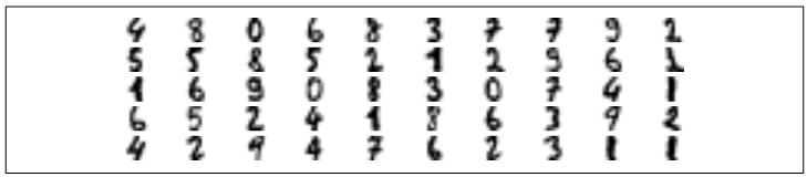
Now let’s look at each image and manually label it:

y_representative_digits = np.array([4, 8, 0, 6, 8, 3, ..., 7, 6, 2, 3, 1, 1])

Now we have a dataset with just 50 labeled instances, but instead of being completely random instances, each of them is a representative image of its cluster. Let’s see if the performance is any better:

log_reg = LogisticRegression()
log_reg.fit(X_representative_digits, y_representative_digits)
log_reg.score(X_test, y_test)

0.9244444444444444

Wow! We jumped from 82.7% accuracy to 92.4%, although we are still only training the model on 50 instances. Since it is often costly and painful to label instances, especially when it has to be done manually by experts, it is a good idea to label representative instances rather than just random instances. But perhaps we can go one step further: what if we propagated the labels to all the other instances in the same cluster? This is called label propagation:

y_train_propagated = np.empty(len(X_train), dtype=np.int32)
for i in range(k):
 y_train_propagated[kmeans.labels_==i] = y_representative_digits[i]

Now let’s train the model again and look at its performance:

log_reg = LogisticRegression()
log_reg.fit(X_train, y_train_propagated)
log_reg.score(X_test, y_test)

0.9288888888888889

We got a tiny little accuracy boost. Better than nothing, but not astounding. The problem is that we propagated each representative instance’s label to all the instances in the same cluster, including the instances located close to the cluster boundaries, which are more likely to be mislabeled. Let’s see what happens if we only propagate the labels to the 20% of the instances that are closest to the centroids:

percentile_closest = 20
X_cluster_dist = X_digits_dist[np.arange(len(X_train)), kmeans.labels_]
for i in range(k):
 in_cluster = (kmeans.labels_ == i)
 cluster_dist = X_cluster_dist[in_cluster]
 cutoff_distance = np.percentile(cluster_dist, percentile_closest)
 above_cutoff = (X_cluster_dist > cutoff_distance)
 X_cluster_dist[in_cluster & above_cutoff] = -1
partially_propagated = (X_cluster_dist != -1)
X_train_partially_propagated = X_train[partially_propagated]
y_train_partially_propagated = y_train_propagated[partially_propagated]

Now let’s train the model again on this partially propagated dataset:

 log_reg = LogisticRegression()
log_reg.fit(X_train_partially_propagated, y_train_partially_propagated)
log_reg.score(X_test, y_test)
#0.9422222222222222

Nice! With just 50 labeled instances (only 5 examples per class on average!), we got 94.2% performance, which is pretty close to the performance of logistic regression on the fully labeled digits dataset (which was 96.7%). This is because the propagated labels are actually pretty good, their accuracy is very close to 99%:

np.mean(y_train_partially_propagated == y_train[partially_propagated])
0.9896907216494846

Suggestions For Reading

To continue improving your model and your training set, the next step could be to do a few rounds of active learning: this is when a human expert interacts with the learning algorithm, providing labels when the algorithm needs them. There are many different strategies for active learning, but one of the most common ones is called uncertainty sampling:

• The model is trained on the labeled instances gathered so far, and this model is used to make predictions on all the unlabeled instances.
• The instances for which the model is most uncertain (i.e., when its estimated probability is lowest) must be labeled by the expert.
• Then you just iterate this process again and again, until the performance improvement stops being worth the labeling effort.

Other strategies include labeling the instances that would result in the largest model change, or the largest drop in the model’s validation error, or the instances that different models disagree on (e.g., an SVM, a Random Forest, and so on).

Next Steps

Before we move on to Gaussian mixture models, let’s take a look at DBSCAN, another popular clustering algorithm that illustrates a very different approach based on local density estimation. This approach allows the algorithm to identify clusters of arbitrary shapes.