Hierarchical Clustering in Machine Learning

K-Means Clustering

• We learned about the K-Means Clustering Algorithm, which finds the centroid of the clusters
• Initialize centroids at random
• Assign observations to the cluster of the nearest centroid
• Recalculate the centroids based on the cluster assignment
• Repeat Steps 2 and 3 until the cluster assignments stop changing

K-Means: Limitations

It is an iterative based approach that requires us to specify the number of clusters.

• Determining the optimal number of clusters can be challenging, especially in cases where the data’s underlying structure is not well understood.
• Final results can be sensitive to the initial placement of cluster centroids and the choice of the distance metric.
• Assumes that clusters are spherical and isotropic, meaning they have similar sizes and densities in all directions.
• Sensitive to outliers, where outliers can disproportionately influence the position of centroids, leading to suboptimal clustering results.

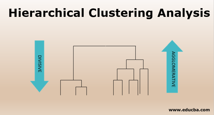
Hierarchical Clustering

• Hierarchical Clustering – An alternative approach that does not require a pre-specified choice of K, and provides a deterministic answer
  • It is based on distances between the data points in contrast to K-means, which focuses on distance from the centroid
  • Agglomerative/Bottom-Up Clustering: We recursively merge similar clusters
  • Divisive / Top-down Clustering: We recursively sub-divide into dissimilar sub clusters.

Agglomerative Clustering

• Start with each point in its own cluster
• Identify the two closest clusters (Ci,Cj)- merge them
  • Repeat until all points are in a single cluster
  • Set threshold t to 0.
  • t = t + e ; where e is a small positive quantity.
  • If the distance between any pair of clusters is < 𝜏, combine them
  • Update all distances from/to the newly formed cluster

To visualize the results we can look at the corresponding dendrogram

Agglomerative Clustering

• The agglomerative clustering is based on the measurement of the cluster similarity.
  • How do we measure distance between a cluster and a point?
  • How do we measure distance between the two clusters?
• The choice of how to measure distances between clusters is called the linkage.
• Linkage is a dissimilarity measure d(Ci,Cj )between two sets of clusters C1 and C2 telling us how different the points in these sets are.
• Different Types:
  • Single Linkage: Smallest of the distance between pairs of samples
  • Complete Linkage: Largest of the distance between pairs of samples
  • Average Linkage: Average of the distance between pairs of samples

Single Linkage

Single linkage also known as nearest-neighbour linkage measures the dissimilarity between C1 and C2, by looking at the smallest dissimilarity between two points in C1 and C2.

Pros: Can accurately handle non-elliptical shapes.
Cons:

• Sensitive to noise and outliers.
• May yield long extended clusters, with point in clusters being quite dissimilar [Chaining]

Complete Linkage

Complete linkage also known as furthest-neighbour linkage measures the dissimilarity between C1 and C2 by looking at the largest dissimilarity between two points in C1and C2.

Pros: Less sensitive to noise and outliers.

Cons:Points in one cluster may be closer to points in another cluster than to any of its own cluster [Crowding]

Complete Linkage

Average Linkage

In average linkage the dissimilarity between C1 and C2, is the average dissimilarity over all points in C1 and C2.

• Tries to strike a balance.
• Clusters tend to be relatively compact and relatively far apart.

Single-Link vs. Complete-Link Clustering

Example of Chaining and Crowding

Single linkage reproduces long chain like clusters, while Complete linkage strives to find compact clusters

Comments on Average Linkage

The average linkage is not invariant to increasing or decreasing transformations of the dissimilarity matrix d

Dendrograms: Visualizing the Clustering

• A 2-D diagram with all samples arranged along x-axis.
• y-axis represents the distance threshold t.
• Each sample/cluster has a vertical line until the threshold t at which they join

Dendrograms

• Dendograms gives a visual representation of the whole hierarchical clustering process.
  • Allows the user to make the final decision
• Applicable irrespective of the dimensionality of the original samples
• One can create multiple clustering based on the choice of threshold
• Can be used with any distance metric and cluster distance measurement strategy (single, complete, average)
• Effective and intuitive cluster validity measure.

K measure from Dendrogram

Outlier Detection With Dendrogram

The single isolated branch is suggestive of a data point that is very different to all others

Lifetime and Cluster Validity

• Lifetime •
  • The time (T𝟐-T𝟏) from birth to death of a specific set of clusters
  • The interval of during which a specific clustering prevails
• Larger lifetime indicates that the clusters are stables over a larger range on distance threshold and hence more valid.

Divisive Clustering

Divisive Clustering groups data samples in a top-down fashion

Divisive Clustering

• Start with all data in one cluster
• Repeat until all clusters are singletons/until no dissimilarity remains between clusters1)

1. Choose one cluster Ck with the largest dissimilarity among its datapoints

1. Divide the selected cluster into two subclusters using different splitting criteria, such as partitioning the cluster along the dimension that maximizes the inter-cluster dissimilarity or using clustering algorithms like K-means to partition the cluster.
2. Update the cluster structure by replacing the original cluster with the two newly formed subclusters.
3. Repeat steps 1-3 until a stopping criteria is met.

Agglomerative vs. Divisive

Agglomerative Clustering

• Bottom-Up Approach
• Computationally Efficient
• Robustness to initialization
• Ease of Interpretation
• Chaining Effect
• Sensitivity to distance metric

Divisive Clustering

• Top-down Approach
• Computationally Expensive
• Sensitivity to Initialization
• Potential for Global OptimumLess Sensitive to Local Structure
• Difficulty in Handling Noise

Hierarchical Clustering: Notes

• Generalizes the clustering process to a hierarchy of cluster labels, which is an inherent nature of the real-world
• We looked into a few basic, yet effective ones
  • Improvements: BIRCH (scalable), ROCK (categorical), CHAMELEON
• Cluster validity allows one to select a specific slice of the hierarchy of clusters
• The approaches need a distance/similarity function between a pair of samples (need not be a simple metric like Euclidean)
• Sensitive to outliers and distance metrics.