
In Previous blog we talked about Non Linear SVM Classifications. In this blog we will talk about Polynomial Kernel.
Introduction
Adding polynomial features is simple to implement and can work great with all sorts of Machine Learning algorithms (not just SVMs), but at a low polynomial degree it cannot deal with very complex datasets, and with a high polynomial degree it creates a huge number of features, making the model too slow.
Fortunately, when using SVMs you can apply an almost miraculous mathematical technique called the kernel trick (it is explained in a moment). It makes it possible to get the same result as if you added many polynomial features, even with very high degree polynomials, without actually having to add them. So there is no combinatorial explosion of the number of features since you don’t actually add any features. This trick is implemented by the SVC class. Let’s test it on the moons dataset.
from sklearn.svm import SVC
poly_kernel_svm_clf = Pipeline([
 ("scaler", StandardScaler()),
 ("svm_clf", SVC(kernel="poly", degree=3, coef0=1, C=5))
 ])
poly_kernel_svm_clf.fit(X, y)
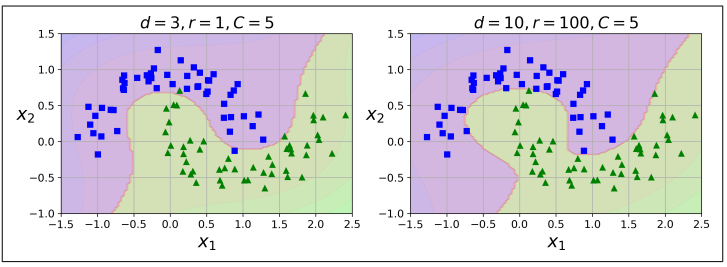
This code trains an SVM classifier using a 3rd-degree polynomial kernel. It is represented on the left . On the right is another SVM classifier using a 10th degree polynomial kernel. Obviously, if your model is overfitting, you might want to reduce the polynomial degree. Conversely, if it is underfitting, you can try increasing it. The hyperparameter coef0 controls how much the model is influenced by high degree polynomials versus low-degree polynomials.
A common approach to find the right hyperparameter values is to

use grid search (see Chapter 2). It is often faster to first do a very

coarse grid search, then a finer grid search around the best values

found. Having a good sense of what each hyperparameter actually

does can also help you search in the right part of the hyperparame‐

ter space.
Adding Similarity Features
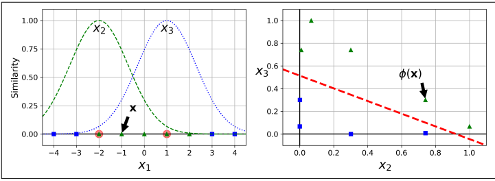
Another technique to tackle nonlinear problems is to add features computed using a similarity function that measures how much each instance resembles a particular landmark. For example, let’s take the one-dimensional dataset discussed earlier and add two landmarks to it at x1
= –2 and x1= 1 .
Next, let’s define the similarity function to be the Gaussian Radial Basis Function (RBF) with γ = 0.3

It is a bell-shaped function varying from 0 (very far away from the landmark) to 1 (at the landmark). Now we are ready to compute the new features. For example, let’s look at the instance x1= –1: it is located at a distance of 1 from the first landmark, and 2 from the second landmark. Therefore its new features are x2 = exp (–0.3 × 12) ≈ 0.74 and x3= exp (–0.3 × 22) ≈ 0.30.
The plot on the right shows the transformed dataset (dropping the original features). As you can see, it is now linearly separable.
Conclusion
You may wonder how to select the landmarks. The simplest approach is to create a landmark at the location of each and every instance in the dataset. This creates many dimensions and thus increases the chances that the transformed training set will be linearly separable. The downside is that a training set with m instances and n features gets transformed into a training set with m instances and m features (assuming you drop the original features). If your training set is very large, you end up with an equally large number of features