Training a machine learning model is, at its core, a search problem.
Your model starts with random weights and tries to find a configuration that minimizes the loss function. Gradient descent provides the direction, but the learning rate determines how far the optimizer moves in that direction.
And that creates a fundamental problem.
Take steps that are too small, and training becomes painfully slow. Worse, the optimizer may get trapped in an undesirable region.
Take steps that are too large, and the optimizer may keep jumping across the minimum without ever settling there.
The solution is deceptively simple:
Start with large steps. Gradually make them smaller.
This is the intuition behind learning rate decay.
The Learning Rate Is Your Step Size
Suppose you are standing on a mountain and want to reach the bottom.
You cannot see the entire landscape. All you know is the direction of the steepest descent immediately around you.
Gradient descent behaves similarly.
The basic update rule is:

where:
- θt: model parameters at step t
- θt+1: updated model parameters
- η: learning rate
- L(θt): loss function evaluated at the current parameters
- ∇L(θt): gradient of the loss with respect to the parameters
The gradient tells the optimizer which direction to move.
The learning rate tells it how far to move.
That distinction becomes extremely important during training.
Why Start With a High Learning Rate?
Imagine your model has just started training.
Its weights are essentially random.
At this point, the optimizer has a huge parameter space to explore.
If the learning rate is extremely small, every update looks like this:
Move a tiny bit.
Check the loss.
Move another tiny bit.
Check again.
The optimizer can spend thousands of iterations slowly crawling through parameter space.
A larger learning rate allows it to cover much more ground.
Large updates can help the optimizer:
- move quickly away from poor initialization
- cross relatively flat regions
- escape small undesirable basins
- explore different regions of the loss landscape
- make meaningful progress early in training
This is particularly useful with stochastic optimization.
Because SGD and its variants already contain noise from mini-batches, a relatively large learning rate can produce a trajectory that is somewhat turbulent rather than perfectly smooth.
That turbulence isn’t necessarily a problem.
Early in training, exploration is valuable.
But Large Steps Eventually Become a Problem
Now imagine the optimizer has reached a promising region.
The loss is already relatively low.
The problem has changed.
You no longer need to travel across the landscape.
You need to fine-tune your position.
Consider a narrow valley:
        \          /
         \        /
          \      /
           \    /
            \  /
             \/
             ●
The bottom of the valley represents a low-loss region.
If the learning rate is too large, the optimizer can jump from one side to the other:
      ●              ●
       \            /
        \          /
         \        /
          \      /
           \    /
            \  /
             \/
Instead of smoothly approaching the minimum, it keeps overshooting it.
The optimizer may oscillate.
In extreme cases, it can even become unstable and cause the loss to diverge.
This is why a learning rate that works well at the beginning of training may be completely inappropriate near the end.
The Training Problem Is Really Two Problems
This gives us an important insight.
Training has two different phases:
Phase 1: Exploration
You want the optimizer to move quickly.
Large learning rate → large updates → faster exploration
Phase 2: Refinement
You want the optimizer to make increasingly precise adjustments.
Small learning rate → small updates → more precise convergence
Trying to use one learning rate for both phases is often inefficient.
That’s why learning rate schedules exist.
Learning Rate Decay
Learning rate decay simply means that the learning rate decreases as training progresses.
Conceptually:
Learning Rate
High  |████████████
      |          ████
      |             ███
      |                ██
      |                  █
Low   |___________________
          Training →
The optimizer starts aggressively and gradually becomes more conservative.
A simple schedule might look like:

where:
- ηt: value of η at time t
- η0: initial value
- γ: decay factor
- t: time or training step
But there isn’t just one way to decay the learning rate.
Several schedules are commonly used.
1. Step Decay
Step decay keeps the learning rate constant for a while and then suddenly reduces it.
For example:
Epochs:       0       30       60       90
Learning rate:
             0.001    0.0005   0.00025  0.000125
The learning rate might be multiplied by a fixed factor every few epochs.
Conceptually:
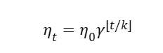
where (k) determines how frequently the learning rate changes.
Why use it?
It’s simple and predictable.
You can essentially tell the optimizer:
Explore aggressively for a while, then slow down.
2. Exponential Decay
Instead of making sudden drops, exponential decay continuously reduces the learning rate.
For example:
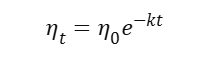
The curve looks more like:
Learning Rate
|
|\
| \
|  \
|   \
|    \__
|       \____
|______________ Training
This creates a smoother transition from exploration to refinement.
3. Cosine Annealing
Cosine annealing uses a cosine-shaped schedule to gradually reduce the learning rate.
A common formulation is:

The important idea isn’t memorizing the equation.
It’s understanding the behavior.
The learning rate starts relatively high and gradually decreases toward a minimum.
This makes cosine schedules particularly popular in modern deep learning training.
Learning Rate Decay Is Similar to Simulated Annealing
There is an interesting analogy here.
In metallurgy, annealing involves heating a material so that its atoms can move and reorganize, followed by gradual cooling that allows the material to settle into a more stable structure.
Optimization has a similar intuition.
At the beginning:
High learning rate → more movement and exploration
Later:
Low learning rate → more stability and refinement
The analogy isn’t exact — learning rate decay is not literally simulated annealing — but the conceptual similarity is useful:
Explore broadly first. Stabilize later.
Why Not Just Use a Small Learning Rate From the Beginning?
You might wonder:
If a small learning rate helps convergence, why not use it throughout training?
Because the optimizer doesn’t know where the good solution is yet.
Suppose the parameter space looks roughly like this:
Starting point
      ●
      |
      |       ______
      |      /      \
      |     /        \
      |____/          \____
                       ↓
                    Minimum
If your steps are tiny, reaching that distant low-loss region can take an enormous number of iterations.
A larger learning rate allows the optimizer to move across the landscape much faster.
So the goal isn’t:
“Find the smallest possible learning rate.”
The goal is:
“Use the right learning rate for the current stage of optimization.”
Why Not Keep the Learning Rate Large?
Because eventually you need precision.
Imagine trying to park a car using only large steering corrections.
You might get close to the parking spot quickly.
But once you’re near the target, those large corrections make it difficult to position the car accurately.
Optimization behaves similarly.
A large learning rate is excellent for making progress when you’re far away.
A small learning rate is better when you’re close.
A Simple Mental Model
Think of learning rate decay as walking toward a target.
At the beginning, take large steps:
“I’m far away. Move quickly.”
As you approach:
“I’m getting closer. Reduce the step.”
Near the target:
“Make tiny adjustments.”
That is essentially what learning rate decay does.
Far from optimum
      ↓
Large steps
      ↓
Fast exploration
      ↓
Promising region
      ↓
Smaller steps
      ↓
Fine adjustments
      ↓
Convergence
Learning Rate Decay in PyTorch
In PyTorch, learning rate schedules are usually attached to an optimizer.
For example:
import torchoptimizer = torch.optim.Adam( model.parameters(), lr=1e-3)scheduler = torch.optim.lr_scheduler.StepLR( optimizer, step_size=10, gamma=0.1)for epoch in range(50): train_one_epoch(model, optimizer) scheduler.step() print( f"Epoch {epoch}: " f"LR = {optimizer.param_groups[0]['lr']}" )
Here, the learning rate is reduced by a factor of 10 every 10 epochs.
You can also use cosine annealing:
scheduler = torch.optim.lr_scheduler.CosineAnnealingLR( optimizer, T_max=50)
The optimizer handles the parameter updates while the scheduler controls how aggressively those updates are made.
But There’s a Deeper Point
Learning rate decay isn’t just a trick for making training converge.
It changes the behavior of the optimization process.
Early training benefits from movement.
Late training benefits from stability.
That’s why learning rate schedules often work better than treating the learning rate as a fixed constant.
The optimizer’s job changes over time.
At first, it is essentially asking:
“Where should I go?”
Later, it is asking:
“How do I fine-tune this solution?”
Those are fundamentally different questions.
One Important Correction to the “Local Minimum” Story
You’ll often hear that a high learning rate prevents SGD from getting trapped in local minima.
That intuition is useful, but it is an oversimplification for modern deep neural networks.
Deep learning loss landscapes are typically extremely high-dimensional and can contain saddle points, flat regions, sharp regions, and many equivalent or near-equivalent solutions.
So it’s better to think of learning rate decay as controlling the balance between:
exploration and refinement
rather than simply:
escaping local minima and finding the global minimum.
This distinction matters when reasoning about optimization in modern neural networks.
The Bigger Picture
Learning rate decay works because optimization is not equally difficult throughout training.
Early on, you need speed.
Later, you need precision.
A fixed learning rate forces the optimizer to make the same-sized decisions throughout the entire journey.
A schedule allows the optimizer to adapt its behavior.
That’s the real idea behind learning rate decay:
Don’t use the same step size when you’re searching for the destination and when you’re standing next to it.
Large steps help you explore the landscape.
Small steps help you settle into a good solution.
And the learning rate schedule is the mechanism that transitions between those two modes.
Final Takeaway
If you remember only one thing, remember this:
Learning rate decay turns optimization from a sprint into a controlled landing.
Start aggressively enough to explore.
Slow down as you approach a promising region.
Finish with small enough updates to converge without constantly overshooting.
That’s why schedules such as step decay, exponential decay, and cosine annealing remain fundamental tools in deep learning.
The optimizer doesn’t just need to know where to go.
It also needs to know when to slow down.
Author
Ved Prakash(LinkedIn)
Senior Data Scientist | AI Engineer | Generative AI
Writing practical tutorials on RAG, LLMs, AI Agents, LangGraph, MCP, Machine Learning, and production AI systems.